
This post is a part of Rethink Priorities' Worldview Investigations Team's CURVE Sequence: "Causes and Uncertainty: Rethinking Value in Expectation." The aim of this sequence is twofold: first, to consider alternatives to expected value maximisation for cause prioritisation; second, to evaluate the claim that a commitment to expected value maximisation robustly supports the conclusion that we ought to prioritise existential risk mitigation over all else.
Executive Summary
Background
- This report builds on the model originally introduced by Toby Ord on how to estimate the value of existential risk mitigation.
- The previous framework has several limitations, including:
- The inability to model anything requiring shorter time units than centuries, like AI timelines.
- A very limited range of scenarios considered. In the previous model, risk and value growth can take different forms, and each combination represents one scenario
- No explicit treatment of persistence –– how long the mitigation efforts’ effects last for ––as a variable of interest.
- No easy way to visualise and compare the differences between different possible scenarios.
- No mathematical discussion of the convergence of the cumulative value of existential risk mitigation, as time goes to infinity, for all of the main scenarios.
- This report addresses the limitations above by enriching the base model and relaxing its key stylised assumptions.
What this report offers
- There are many possible risk structure and value trajectory combinations. This report explicitly considers 20 scenarios.
- The report examines several plausible scenarios that were absent from the existing literature on the model, like:
- decreasing risk (in particular exponentially decreasing) and Great Filters risk.
- cubic and logistic value growth; both of which are widely used in adjacent literatures, so the report makes progress in consolidating the model with those approaches.
- It offers key visual comparisons and illustrations of how risk mitigation efforts differ in value, like Figure 1 below.
- The report is accompanied by an interactive Jupyter Notebook and a generalised mathematical framework that can, with minor input by the user, cope with any arbitrary value trajectory and risk profile they wish to investigate.
- This acts as a uniquely versatile tool that can calculate and graph the expected value of risk mitigation.
- The user can also adjust all the parameters in the 20 default scenarios.
Takeaways
- In all 20 scenarios, the cumulative value of mitigation efforts converges to a finite number, as the time horizon goes to infinity.
- This implies that it is not devoid of meaning to talk about the amount of long-term value obtained from mitigating risk, even in an infinitely long universe.
- In this context, even if we assign any minuscule credence to one of the scenarios, it won't overshadow the collective view.
- It helps clarify what assumptions would be required for infinite value.
- The report introduces the Great Filters Hypothesis:
- It states that humanity will face a number of great filters, during which existential risk will be unusually high.
- This hypothesis is a more general, and thus more plausible, version of what is commonly discussed under the name ‘Time of Perils’: the one filter case.
- Persistence – the risk mitigation’s duration – plays a key role in our estimates, suggesting that work to investigate this role further, and to obtain better empirical estimates of different interventions’ persistence would be highly impactful. Other tentative lessons:
- Interventions to increase persistence exhibit diminishing returns, and are most valuable for mitigation efforts exhibiting small persistence.
- Great value requires relatively high persistence, and the latter could be implausible.
- It is often assumed that, when considering long-term impact, existential risk mitigation is, in expectation, enormously valuable relative to other altruistic opportunities. There are a number of ways that could prove to be false. One possibility, which this report emphasises, is that the vast value of risk mitigation is only found in certain scenarios, each of which makes a whole host of assumptions.
The expected value of risk mitigation therefore strongly depends on our beliefs about these assumptions. And, depending on how we decide to aggregate our credences and which scenarios we allow for, astronomical value might be off the table after all.
Figure 1 (see header's image): This is a visual representation of the estimated expected value of reducing existential risk by 0.01%. The image is to scale and one cubic unit is the size of the world under constant risk and constant value, the top-left scenario.
This abridged technical report is accompanied by an interactive Jupyter Notebook. The full report is available here.
Recommended: The PDF version of the abridged report can be accessed here.
Abridged Report
Introduction
Consider a catastrophe that permanently ends human civilisation.[1] You might find it plausible that any efforts to reduce the risk of such a catastrophe are of enormous value. You might also be inclined to think that the value is particularly high if the risks are high also. After all, in most contexts, the bigger the risk of something bad happening, the less it can be safely ignored. In other words, you might believe that it is of astronomical importance to mitigate these extinction risks because the stakes are very large and because the probability of these catastrophic scenarios is uncomfortably high. Existing work by Ord, Adamczewski and Thorstad (hereon 'OAT') argues that this last sentence is questionable: in the context of an extinction catastrophe, the higher we think the risk is, the less we should value efforts that mitigate that risk.[2]
Our initial intuitions are not always a good guide for how we should think about estimating the value of extinction risk mitigation. Indeed, the unexpected tensions between high pessimism about the risk we face and whether risk mitigation is of astronomical value, are a good example of this.[3] Similarly, simplified attempts and heuristics used to estimate the cost-effectiveness of risk reduction ---- such as those in 1, 2, 3, 4, 5 ---- turn out to only be appropriate in a handful of very restricted scenarios (usually where value and risk are constant in all the periods), and they otherwise mischaracterise the value of extinction risk mitigation.
If we want to evaluate the general merits of interventions that seek to safeguard humanity's future, we need a systematic way to estimate the value of mitigating extinction risk. The current frameworks help us understand which scenarios might lead to astronomical value. However, they have several limitations that make it difficult, or sometimes impossible, to comment meaningfully on the amount of good that mitigating risk in the next few decades could achieve. This report builds on the existing models and provides tools to estimate the value of mitigating risk in more realistic settings.
The Base Model
As a first attempt to provide a more rigorous analysis, existing work presents a stylised model to assess the value of extinction risk mitigation given the following assumptions:
A1 Each century of human existence has some constant value.
A2 Humans face a constant level of per-century extinction risk.
A3 No value will be realised after an extinction catastrophe.
A4 Risk is reduced by a fraction.
A5 Risk is only reduced this century.
A6 Centuries are the shortest time units.
The model is clearly oversimplified, and, indeed, previous work has partially relaxed a subset of these six assumptions.[4] However, there are still several limitations present in those frameworks.
OAT Limitations
Some of the main limitations of the previous work include:
- The current models lack the necessary resolution to yield results that are relevant for, or incorporate observations from, key issues like near-term AI timelines. The models cannot presently handle anything requiring shorter time units than centuries.
- The duration of a mitigation action's effects affects its overall value. However, OAT has not explored how varying the duration of these effects may impact the model.[5]
- There are many possible scenarios (i.e., combinations of risk and value trajectories), and OAT has explored very few of these. Given our large uncertainty in this area, it is a priority to have a clear picture of how the value compares in each case. This will provide the necessary tools for future work that assigns credences to each scenario to arrive at better-informed expected value judgements.
- There are currently no versatile frameworks that can calculate the expected value of mitigating risk, for a given set of idiosyncratic beliefs about risk and value trajectories.
- As time goes to infinity, the expected value of existential risk mitigation could, in principle, be infinite; making most scenario comparisons redundant in those cases. There has been no formal discussion of the convergence of the value of extinction risk mitigation for all of the main scenarios.
Key Research Questions
The present report aims to tackle all of the above limitations. With that in mind, the key guiding questions are:
- When is the value -- of the future and of risk mitigation -- particularly large and when is it not?
- What is the Great Filter Hypothesis, how does it relate to the Time of Perils and what is the impact of adding great filters on the value of risk mitigation?
- What are the qualitative pictures of the expected value of the world -- and thus of mitigation efforts -- given different risk structures (e.g. linear, Time of Perils, Great Filters, decaying) and value growth cases (e.g. linear, quadratic, cubic, logistic)?
- How does the value of mitigation efforts depend on their persistence?
The main ambition here is to develop a generalised version of the toy model that relaxes all assumptions above, except for A3, no value after extinction, and A4, fractional risk reduction.[6][7] By relaxing A1 and A2 -- that the value and risk are constant -- we are able to introduce a framework that can accommodate more complex risk structures and sophisticated value trajectories. We also depart from existing analyses by relaxing A6: here, years are the shortest time unit. Moreover, by also relaxing A5, the model now has tools to observe persistence of mitigation effects lasting less (or more) than one century and can meaningfully comment on the near-term value of extinction risk mitigation. Using this generalised framework, we can systematically assess the value of risk mitigation under various combinations of assumptions.
Generalised Model: Arbitrary Risk Profile
Let us consider the expected value of a world that faces an existential risk at time . This is best observed with a picture.
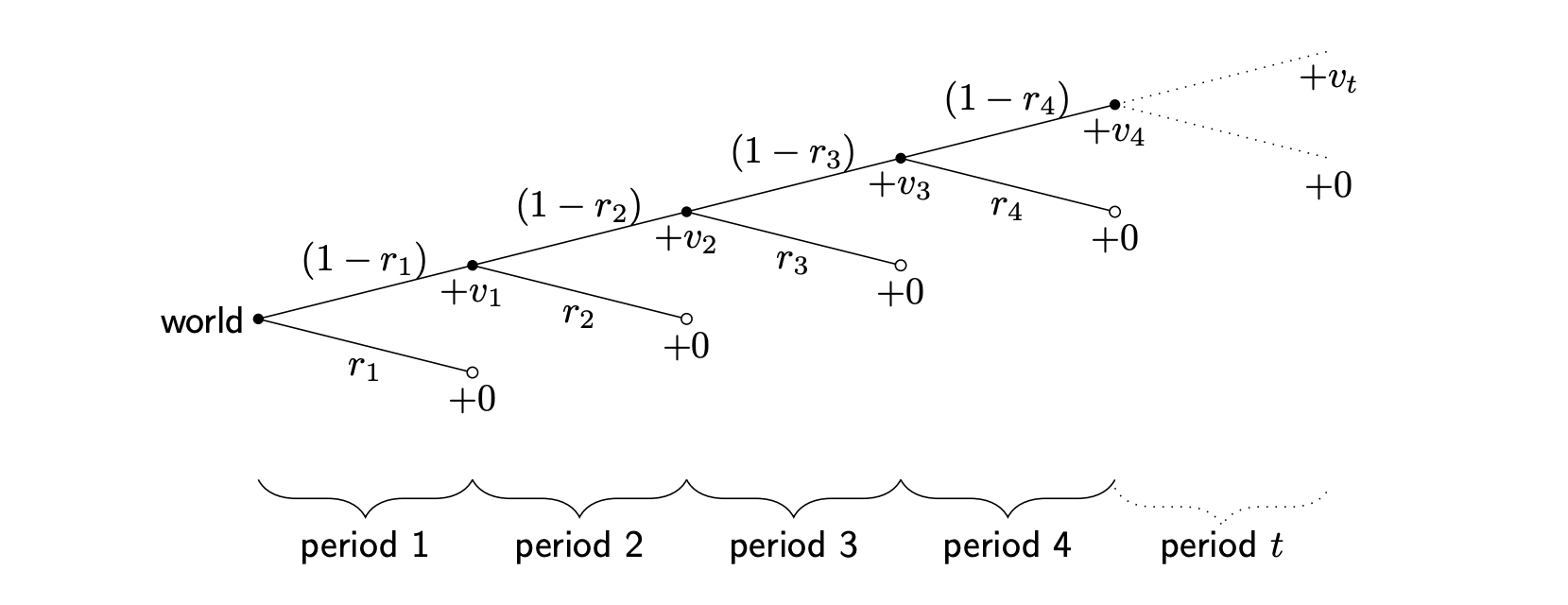
At each period the world ends with probability and all possible future value is reduced to zero. On the other hand, with probability , the world progresses to the next period and achieves value , which is added to the total pool of value it had accrued. Figure 2 summarises all of this. The expected value is the value of each branch weighted by the probability of reaching that value. That is
In other words, the expected value of this world is
[Equation 1]
where the maximum number of periods is the age of the universe when it ends, and when we assume an infinite universe. We do not impose that or otherwise to give the flexibility to consider cases where there is some known, exogenous, end to the universe. Throughout this document, the length of a period will equal one year. However, the results are not tied to any particular interpretation of period length.[8]
Now consider a risk mitigation action which reduces the original risk sequence from to , where, for some , and is the fraction of the risk that is successfully mitigated.[9][10] What value have we added by performing action ? In the most basic sense, we have changed the expected value of the future by
where our action modified the original risk from in world to in .[11] More generally, we could allow , which would amount to increasing the risk and would produce negative value (or none at all if ). For example, if made a nuclear war more likely by contributing to political instability. For the rest of the report we focus on non-negative value.
Value
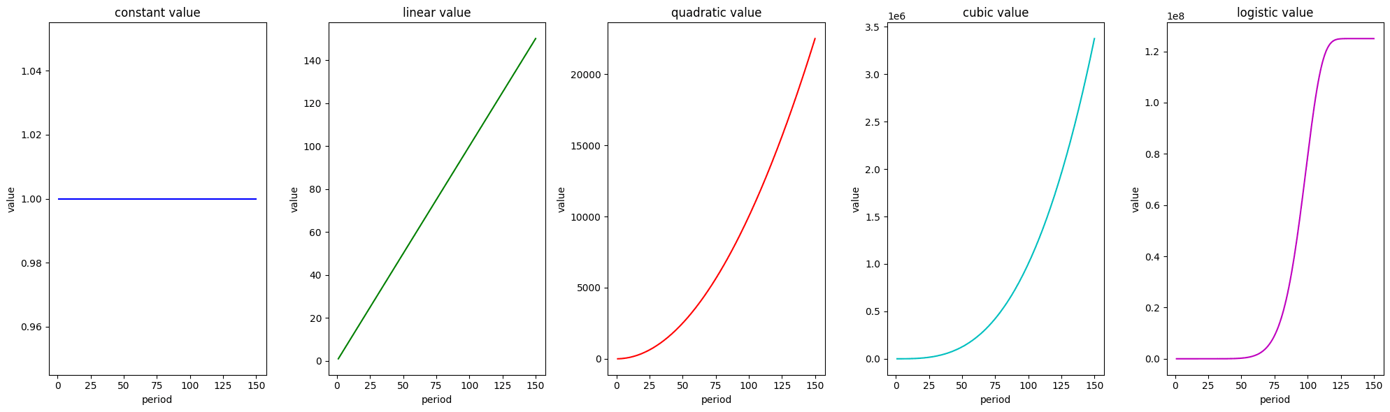
Denote as as the sequence of values that the world will follow, conditional on the world existing at time . Estimating this sequence is no trivial undertaking. There is large uncertainty in this area and considerable research is needed for us to insert reasonable values into the sequence . Given this uncertainty, a promising approach is to develop a more flexible framework, i.e. the generalised model above and its accompanying code in the Jupyter Notebook, that is versatile enough to handle a wide range of cases. Next, we will investigate several possible paths for value growth, in particular: constant, linear, quadratic, cubic and logistic.
Value Cases Summary
Here is a table summary of the main value cases this report will investigate.[12] When the time unit is years instead of centuries, the value is adjusted to reflect this (see the full report here for the details). Cubic has previously been adopted for modelling interplanetary expansion. Logistic can be thought of as 'exponential with a value cap', a model that has special economic relevance.[13]
| Constant | Linear | Quadratic | Cubic | Logistic | |
Table 1: Summary of Cases
Here is a visual summary.
Persistence
Extinction risk mitigation actions could have effects that last different amounts of time. We may have reasons to believe that an action will reduce risks only for a few years; for example, passing a bill that restricts AI compute which is expected to be overturned after the next election cycle in 5 years. Other actions could last longer; for example, a shield in space that physically protects Earth from asteroid impact could be effective for thousands of years. Or, in the extreme case, an action could reduce extinction risk forever. In this report, we refer to the length of the mitigating effect of an action as its persistence.
Persistence is key in evaluating the value of an action . In the Ord model, the persistence of has been assumed to be of exactly one period (which equals one century in that setting). Thorstad proceeds with the same assumption and briefly considers the permanent case as well. Because persistence plays such an important role, we developed a more flexible framework where we allow persistence to be anything between one period and permanently reducing risk, i.e. .
An investigation of persistence likely deserves a report of its own, both for a theoretical and empirical treatment of the issue. For now we will assume that mitigates risk for periods, without delay. We illustrate how results differ by presenting five representative cases: .
So, for example, if we had a risk profile of and acts at the first period with persistence and an efficacy of , halving the risk, the profile then becomes: .
A Concrete Example
There are too many cases for us to explicitly consider each one in the exposition of this report. Instead, they are systematically solved for and implemented in the code; so the user can see the results for any one desired scenario. However, it is pedagogically valuable to explicitly discuss one of these cases here.
Suppose that performing halves the risk with a -year persistence. Let us also add some complexity to the risk structure, so it takes two constant values. Suppose that there is a 0.22% annual risk, which approximates a one in five chance of surviving the end of the century, under the assumption that it remains constant for the next 100 years.[14] Suppose that, for no particular reason, the annual risk after those 100 years is 0.01%.[15] That is . Suppose, for this exercise, that this universe lasts 10,000 years.[16] We also normalise the value unit to . What is the value of performing ? It is
It is worth roughly 28.6 to perform under these assumptions, where is this year's value of our world.
The Rest of this Report
So far, we have thought about risk in the abstract. Indeed, what we have outlined is enough for us to evaluate any arbitrary risk and value structure that we may want to test. See the Jupyter Notebook to try this yourself.
However, there are specific risk structures that we might be especially interested in evaluating. We might be inclined to believe certain stories about risk; for example, that it will systematically decline (like in the Decaying Risk section). Alternatively, we might want to pay heed to the commonly held view that humanity is living in a particularly risky period now, but will reach a low-risk future if it overcomes the present challenges. The concrete example above is an instance of this, assuming constant value. Thorstad states this view, termed the 'Time of Perils' sis and discussed more thoroughly here, as:
(ToP) Existential risk is and will remain high for several years, but it will drop to a low level if humanity survives this Time of Perils.
We explore this type of risk structure next.
Great Filters and the Time of Perils Hypothesis
Humanity is potentially facing unprecedented threats from nuclear weapons, engineered pandemics and advanced artificial intelligence, among others. It may be that we are living in perilous times. If we do well, we might escape these dangers. But who's to say that there will be no comparable challenges in the future? The perilous times might return.
The reasoning above introduces the notion of great filters: hurdles that our civilisation must pass to ensure its long-term longevity (Hanson, 1998).[17] Specific details as to what these filters might be are beyond this work. But if AI is the first filter, we could easily imagine future ones such as escaping our dying sun or meeting powerful and unfriendly alien life. The great filter hypothesis tells us:
(GFH) Humanity will face one or more great filters, during which extinction risk will be unusually high. Otherwise, the risk will be low.
It follows that, by construction, the Time of Perils hypothesis is the one filter version of GFH. For the purposes of this report, let us consider a stylised model of GFH where:
- There are filters (e.g. ).
- There are 'eras', sets of periods within which risk is constant. Filters are high-risk eras.
- Filters and low-risk eras alternate, starting with a filter.
- The length of each era is given by .
- At each era , humanity faces a per-period constant risk , and denotes the vector .
For example, suppose that we had , such that there are two filters, with two lower-risk eras of lower risk after each of them. Suppose that , and that value is constant. From this we could write the expected value of such a world as
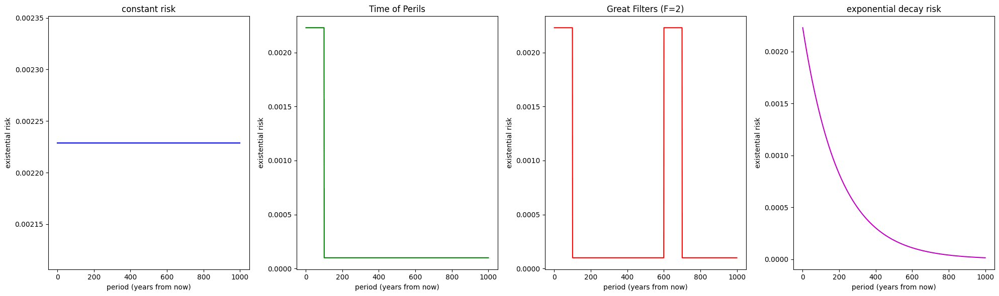
Decaying Risk
Optimistically, we could live in a world where humanity is progressively getting better at surviving. One way of modelling this is with decreasing risk, and in particular, we can specify an exponentially decreasing function; where is the risk as , is the decay rate, is the period, is the risk in period and the starting risk is for small . For the first few periods, the sequence is approximately: More generally,
Risk Cases Summary
A graph summarising the main cases of interest can be found below.
Results
Convergence
As time goes to infinity, the expected value of existential risk mitigation could, in principle, be infinite. This would render comparing different estimates of redundant.[18] To investigate when this might happen, we turn our attention to convergence next.
We know that for any finite , Equation 1 is bounded.[19] A key issue is whether the expected value of the world converges in an infinite universe. When , the series for the expected value of a world, , as described in Equation 1, is given by the infinite sum
For this kind of series, we can use the Ratio Test to evaluate its convergence. The Ratio Test states that for a series , if there exists a limit then the series converges absolutely if , diverges if , and is inconclusive if . To apply the Ratio Test to , we look at consecutive terms of the series and their ratio.
Recall that for all , so also lies within for all . Thus, if converges to a positive scalar, the exact risk level will not affect convergence. Instead, the convergence of the series critically depends on . In particular, we find that this limit is less than or equal to 1 in our cases of interest, thus converges absolutely. The full details can be found in the report but as an example, consider the n-polynomial case, which is a more general version of all the cases, excepting logistic.
Consider the -polynomial case . Then:
Under logistic, also. Hence, in the context of the various scenarios we've explored, we are now ready to present the following result:
Proposition 1. The expected value of the world is finite if existential risk does not converge to zero.
Proof. See the full report. An intuition: asymptotically, the probability of survival shrinks every period by a constant proportion, while value is either constant or increasing polynomially at a shrinking proportion. Therefore the expected value contribution for a distant enough approximates zero. ◻
Maintain the assumption that the risk tends to any nonzero value. As an immediate consequence of the above proposition, we have:
Corollary 1. In an infinitely long universe, the value of existential risk mitigation is finite.
Proof.
and, by Proposition 1, both and converge. ◻
These results, tell us that it is meaningful to talk about the long-term value of risk mitigation, even in the infinite universe case. Moreover, however great the value might be, it is simply not infinite. We estimate the exact size of this value next, in the Results section. It should be emphasised that the scope of Corollary 1 and Proposition 1 is the scenarios that this report considers, and not all the possible ways of modelling risk and value. For example, the proofs fail when the risk exponentially decays to zero, or when value grows exponentially without a cap.
The Expected Value of Mitigating Risk Visualised
First, we present Figure 5, a grid which summarises what the expected value of the future is, without the presence of risk mitigation efforts.
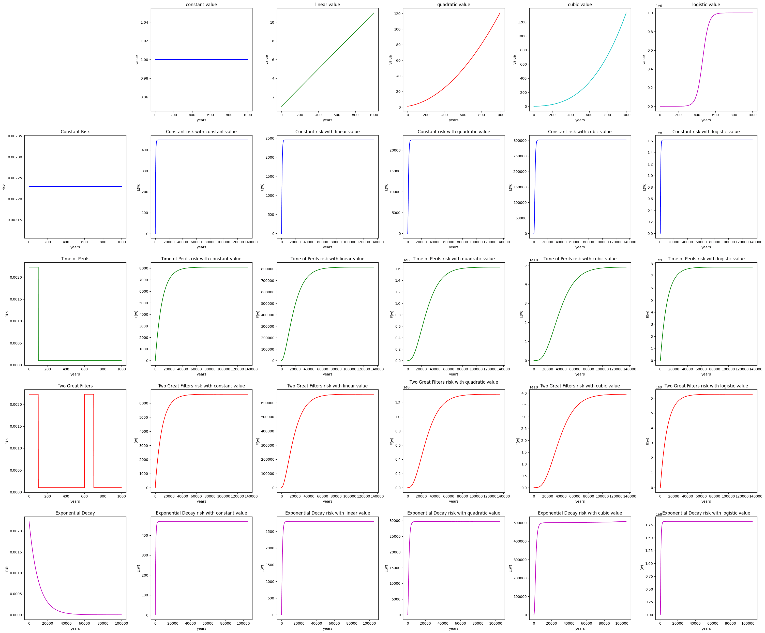
The first column indicates what value case we are on, the first row what risk case, and the middle plots display the cumulative as time passes for each risk and value combination. Notice that in all cases, converges as . This is only indirectly related to the Convergence section, which is about the convergence of and not the expected value of the future. For the middle plots, the horizontal axis displays the range from year zero (today), until year 140,000. For visibility, we display until year 100,000 for exponential decay instead. The vertical axis is different every time so that all graphs are clearly visible. For example, constant risk under linear value is in the thousands of and Two Great Filters under logistic value is in billions of , where is always normalised to one. The default parameters for these simulations can be found and modified in the Notebook.
Next, we plot , with and without performing for all twenty scenarios in Figure 6. We do this for a range of persistence levels and, for entirely pedagogical reasons, we assume an extreme efficacy of reduction in the risk from performing .
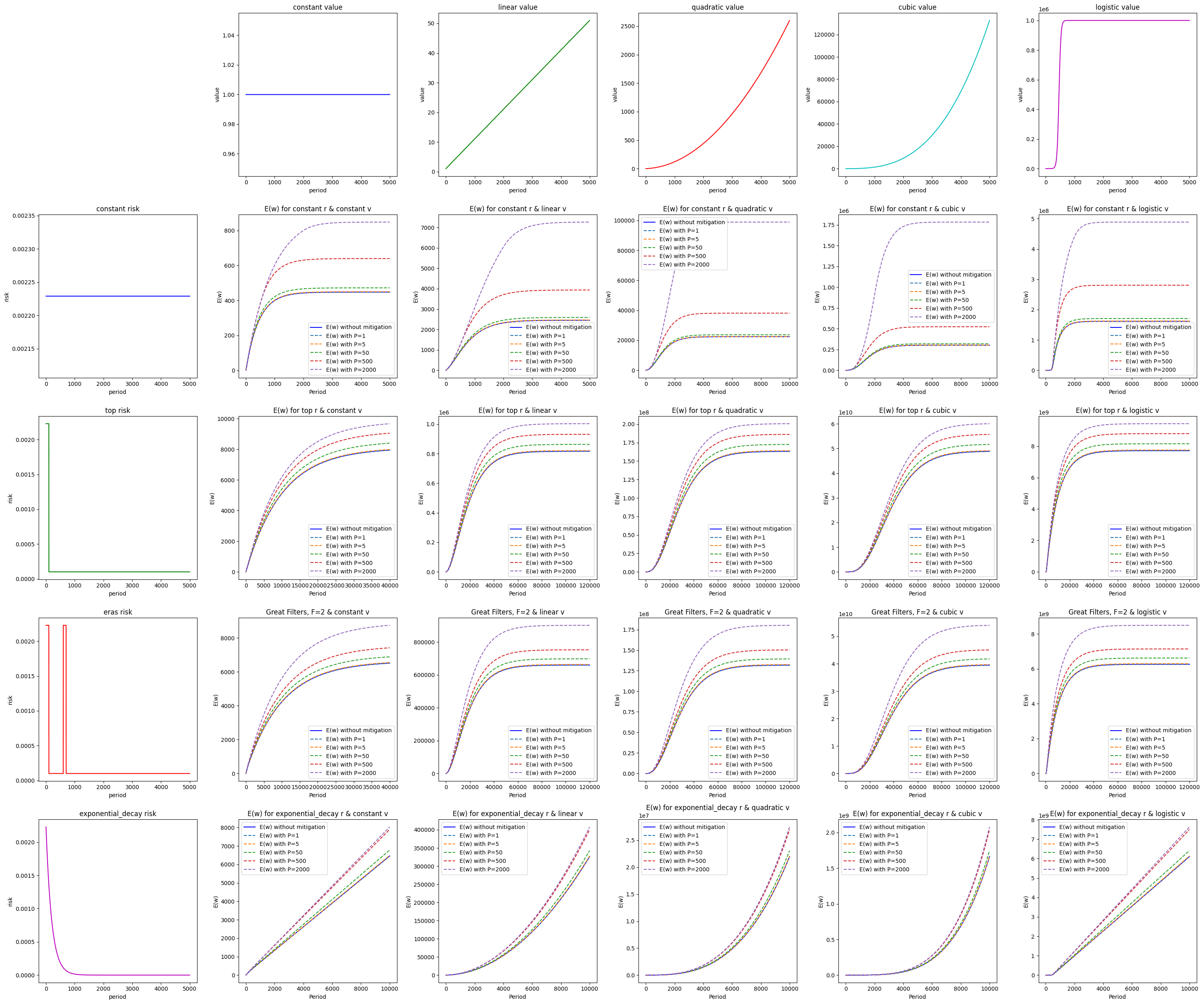
In the grid above, to calculate for some specific case, we first take the dotted curve that tells us the expected value of the world after performing the action, all under a particular scenario and at certain persistence. Then, we subtract the baseline without mitigation, i.e. we subtract the solid blue curve from any one dotted curve.
When discussing the value and eventually the cost effectiveness of risk mitigation, a useful and more realistic efficacy is one basis point: . Table 2 below shows for all the scenarios of interest.
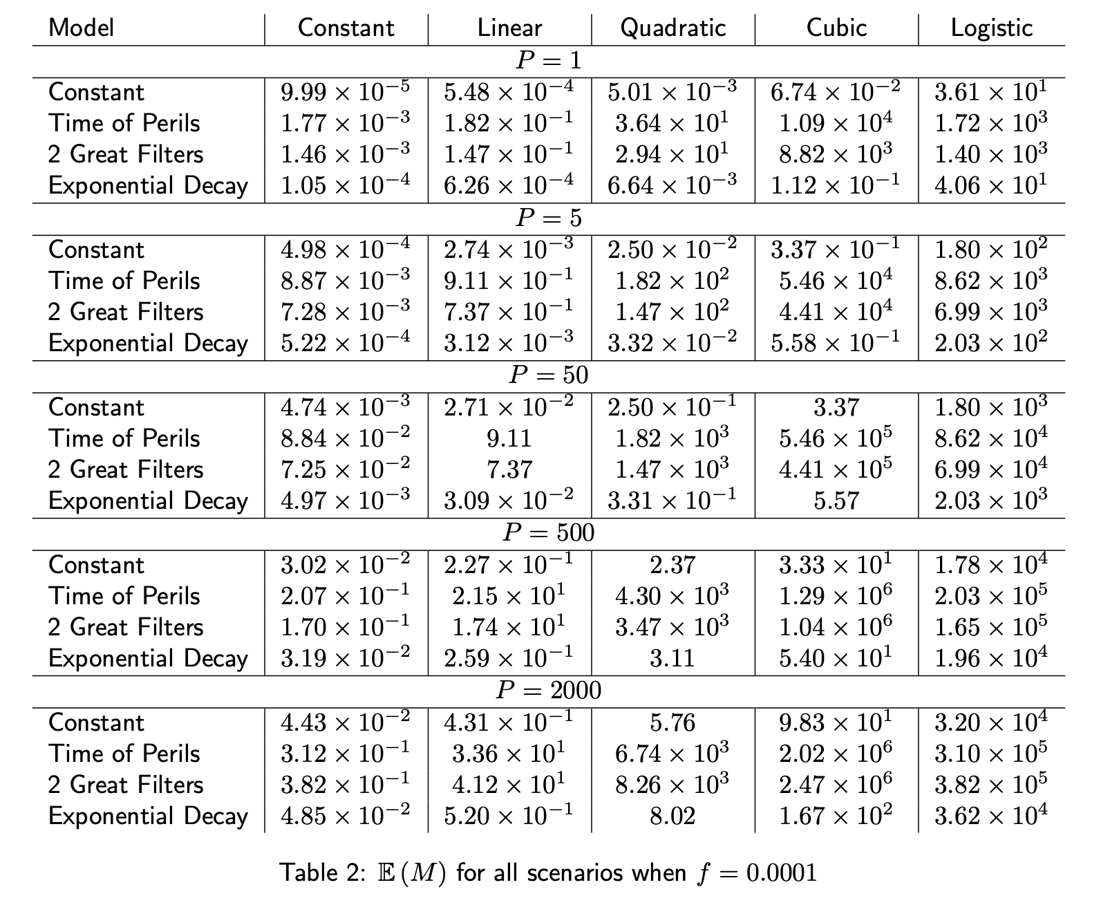
Though we show it above, we are suspicious of long persistence, both because effects are blunted by political or technological changes and because, given enough time, some actor is likely to perform an action that achieves similar effects.[20]
Given the difference in orders of magnitude, it can be difficult to directly compare the figures in this table. To facilitate this, we display Figure 1: a visual representation of the estimated expected value of reducing existential risk by 0.01%.[21] The image is to scale and one cubic unit is the size of the world under constant risk and constant value, the top-left scenario. A persistence of 5 years is assumed.
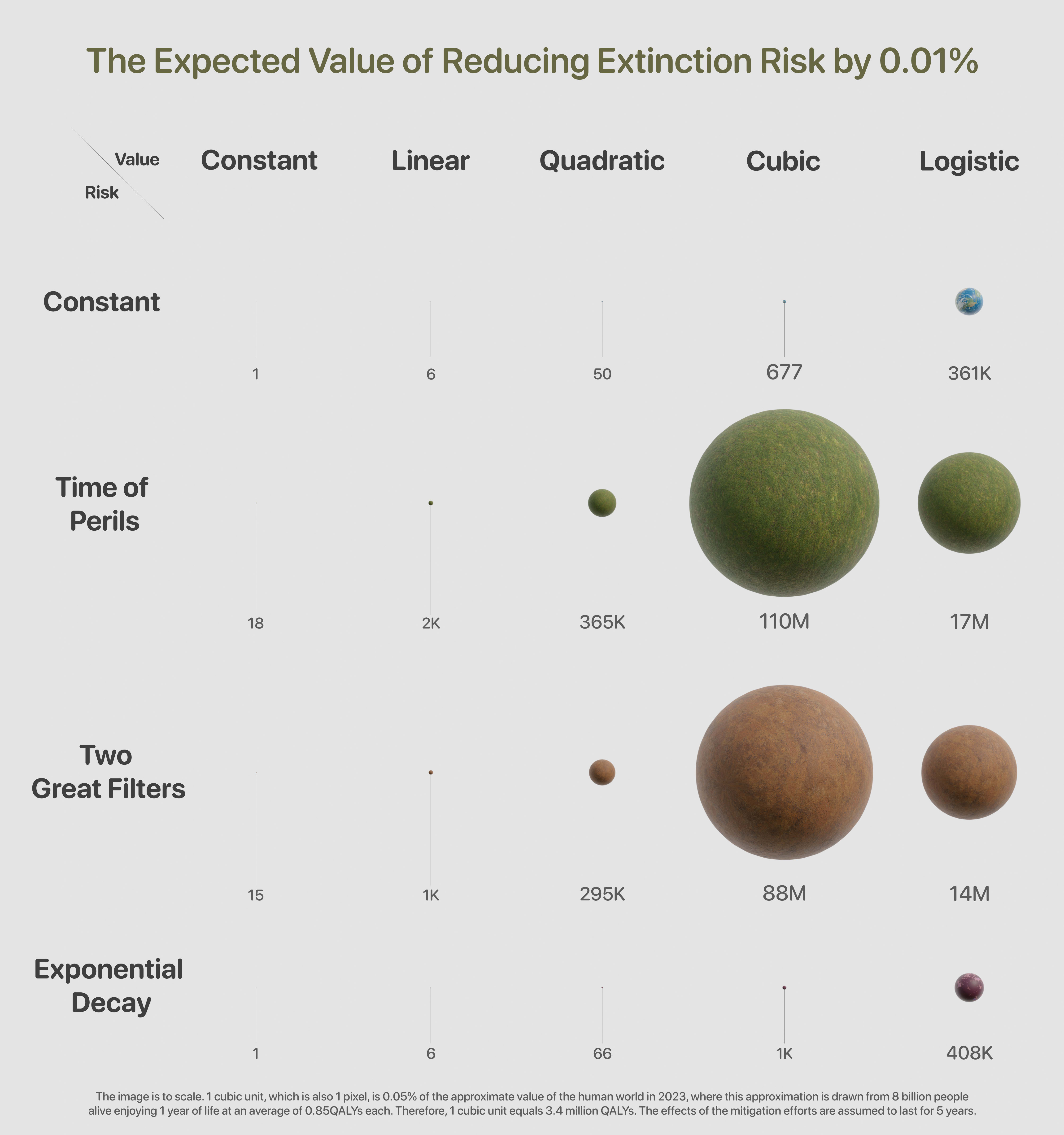
For an extended discussion of these results see the full report. Here are some key takeaways:
- How many orders of magnitude is under Time of Perils crucially depends on assumptions about value growth (it is 11 million times bigger under cubic value compared to constant).
- For constant value, as we vary the assumed risk and persistence, stays within one order of magnitude above or below the median value in Table 2. For linear and quadratic it's within two orders of magnitude.
- Adding another filter keeps in the same order of magnitude, and only reduces it by about 25%, under the default parameters in the Notebook.
- Given a fixed persistence, there's still extreme variability: the minimum is roughly 8 orders of magnitude smaller than the maximum.
- This extreme difference can be put succinctly: suppose that the units were meters travelled as you walk away from London Bridge. The smallest value implies you'd walk 17cm, about the length of a pencil. Whereas the largest means that you'd walk from London to Sydney.
The Role of Persistence
Two remarks seem worth making. First, that persistence plays a key role in the value of risk mitigation. For example, in Figure 7 below, depending on persistence can increase by up to 30 times. Second, we suggest an empirical hypothesis that persistence is unlikely to be higher than 50 years. The reasoning here is that there might be interventions that reduce risk a lot for not very long or not very much but for a long time. But actions that drastically reduce risk and do so for a long time are rare. Jointly these two remarks entail that the value of risk mitigation is between one ten-thousandth of a (under constant risk and value) and two billion (under cubic and time of perils assuming is one basis point), a considerable range.[22]
To illustrate the role of persistence consider the following picture, which plots versus persistence in the constant risk and value case for .
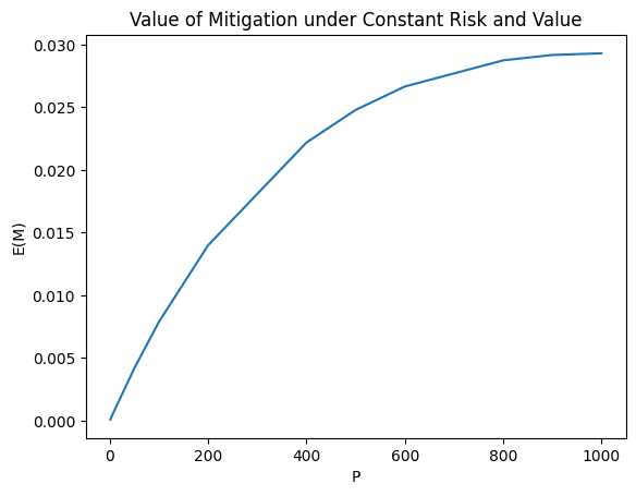
Increasing persistence is important but it exhibits decreasing marginal returns in the concave fashion illustrated above.
This result matches our intuitions. Because of its cumulative nature, the probability of avoiding extinction in the near-term is much higher than avoiding it long-term. That means that the value contributions to , which also impact , are much higher in the short term than in the long term, when they are heavily discounted by the probability of them taking place. So the marginal gains from increasing persistence are much higher in the short term than in the long term. In other words, for example, adding 1 year of persistence to a mitigation action whose effects last 1 year is much more valuable than adding 1 year of persistence to a mitigation action whose effects last 100 years. A general lesson follows: performing actions that have larger persistence is key, but increasing persistence is particularly valuable for low persistence values.
Concluding Remarks
This report is restricted in its scope and has a number of limitations. If there is enough value and interest in this type of work, our follow-up research could include:
- a friendlier online platform with sliders and buttons to select and tweak the scenarios users want to visualise
- explicit closed-form expressions for comparative statics, formulae that describe the impact of shifting key parameters on
- explicit uncertainty analyses with Monte Carlo simulations where we graphically observe the importance of key parameters and different upper and lower bounds of according to a range of scenarios
- more sophisticated treatments of persistence
- discussions about option value and its role in thinking about existential risk mitigation
- modelling efforts that improve value trajectory and could be competitive with extinction risk reduction
- including partial catastrophes
- formally exploring other events conceptually included in existential risk but not extinction risk
- including population growth as a parameter that directly affects values
- new scenarios, including explicit treatment of population growth and other non-human sentience
- investigating value trajectories that feature negative value
With these limitations in mind, some points of caution about practical upshots include:
- Depending on the parameters of exponential decay, and the time horizon, convergence under exponential decay risk can be misleading, check the Jupyter Notebook for full details.[23]
- While the results here might help us arrive at better-informed expected value judgements, this report is not meant to settle questions about how to form an overarching view on the overall value of extinction risk mitigation. A lot more work is needed for that, for instance, our views on risk aversion could play an important role.
- Readers should be careful with using the reports' results to perform back-of-the-envelope calculations with new parameters in mind, and update your views by roughly deducting or adding some orders of magnitude. When possible, rerun the code instead.[24]
- More broadly, while a more complex model like this one can certainly model things that were previously left out, we have so little data to fit it to that we should be especially cautious about over-updating from specific quantitative conclusions.
This report extended the model developed by Ord, Thorstad and Adamczewski. By enriching the base model, we were able to perform sensitivity analyses, observe convergence and can now better evaluate when extinction risk mitigation could, in expectation, be overwhelmingly valuable, and when it is comparable to or of lesser value than the alternatives. Crucially, we show that the value of extinction risk work varies considerably with different assumptions about the relevant risk and value scenarios. Insofar as we don't have much confidence in any one scenario, we should form views that reflect this uncertainty and we shouldn't have much confidence in any particular estimate of the value of risk mitigation efforts.
- ^
Previous work has referred to such a risk as 'existential risk'. But this is a misnomer. Existential risk is technically broader and it encompasses another case: the risk of an event that drastically and permanently curtails the potential of humanity. For the rest of this report we characterise the risk as that of extinction where previous work has used 'existential'.
- ^
The reasoning goes that if there is always a high level of background risk to humanity, then we should expect to go extinct soon anyway, which means the importance of avoiding any one particular risk is not as valuable as it may seem. For more details see the full report here.
- ^
In particular, Thorstad explores how, in this model, extinction risk pessimism fails to support and sometimes hinders the thesis that extinction risk mitigation is of astronomical value.
- ^
For example, Thorstad relaxes each of the A1, A4 and A5 assumptions.
- ^
The models thus far centred around mitigating risk for one century only. Thorstad comments on one additional case: when risk is permanently mitigated, calling it 'global risk reduction'.
- ^
We leave A4 untouched because it introduces diminishing returns in risk reduction (see more the details Adamczewski discusses), which we find realistic.
- ^
A3 is a core assumption in the extended and simplified versions of this model. Relaxing it would amount to changing the approach completely.
- ^
That said, the risk and value trajectories usually need adjusting when considering a different time unit. For more details see the section on adjustments on the full report here.
- ^
In its most general form, could be any new risk vector that has brought about. All there is left to evaluate the value of the action is to compute .
- ^
Alternatively, an altruistic intervention could seek to improve the future by positively influencing the value trajectory; that is, by bringing about a better rather than a new . Such actions, deserve a separate analysis.
- ^
So far we have been writing to abbreviate , where and are, respectively, the risk vector (sometimes termed 'risk profile'), the value vector and the maximum number of periods in our universe, which could be infinite. Note that a different class of interventions might focus on increasing the value of the world from to , which would also result in negative value according to . Exploring these is not within the scope of this report.
- ^
Here: is the value at time , is the cap value the can reach and is the starting value at . is a constant, normalised to 1 in all the simulations. More generally, we interpret as one year of value in , which in human terms is roughly billion people enjoying life at an average of QALYs each.
- ^
Other work, has considered exponential without a cap. There seem to be good reasons to posit a cap, however high, like the physical limits on how much matter is accessible to humans in our expanding universe.
- ^
The probability of dying each year that gives a 0.2 probability of dying over 100 years is approximately 0.00222894771 or 0.22%. To see why, consider the following binary outcomes model. Let be the probability of dying in a given year. The implied probability of surviving for one year is . The probability of surviving for 100 years consecutively would be . Given that there's a 0.2 probability of dying over 100 years, the probability of surviving the entire 100 years is . Thus, .
- ^
Which is congruent with a probability of surviving each century.
- ^
Numerical approximations of the expected value of converge in this setting for large so an infinite universe could be thought of as finite, without loss of generality. See the Convergence section for a discussion of convergence.
- ^
An excellent informal introduction to great filters can be found here.
- ^
Tentatively, ordering infinite cardinalities could be a good option in those cases.
- ^
For example by .
- ^
On the latter point, to calculate the actual difference that our efforts makes to the effects of persistence will require future work. For example, imagine you do an action, , at that mitigates risk for the next 10 years. If you hadn't done , someone else would have taken that same action at . How should we measure the persistence and value of in this case? The treatment of 'contingency' here can help guide our thoughts.
- ^
Because of computational limits, the expected value calculation assumes a cap of 120 thousand years. This is more than long enough in most scenarios, where a this large achieves the same behaviour as , but nuances arise in the exponential decay case, see the notebook for a thorough discussion of those.
- ^
Recall the previous footnote defining .
- ^
In particular, Figure 1's exponential decay values were approximated using the first 100,000 years.
- ^
I'm happy to help with this.
Acknowledgements

The post was written by Arvo Muñoz Morán. Thank you to the members of the Worldview Investigations Team – David Bernard, Hayley Clatterbuck, Bob Fischer, Laura Duffy and Derek Shiller – Marcus Davis, Toby Ord, Elliott Thornley, Tom Houlden, Loren Fryxell, Lucy Hampton, Adam Binks, Jacob Peacock, Daniel Carey for helpful comments and discussions. The post is a project of Rethink Priorities, a global priority think-and-do tank, aiming to do good at scale. We research and implement pressing opportunities to make the world better. We act upon these opportunities by developing and implementing strategies, projects, and solutions to key issues. We do this work in close partnership with foundations and impact-focused non-profits or other entities. If you're interested in Rethink Priorities' work, please consider subscribing to our newsletter. You can explore our completed public work here.
Why are these expected values finite even in the limit?
It looks like this model is assuming that there is some floor risk level that the risk never drops below, which creates an upper bound for survival probability through n time periods based on exponential decay at that floor risk level. With the time of perils model, there is a large jolt of extinction risk during the time of perils, and then exponential decay of survival probability from there at the rate given by this risk floor.
The Jupyter notebook has this value as r_low=0.0001 per time period. If a time period is a year, that means a 1/10,000 chance of extinction each year after the time of perils is over. This implies a 10^-43 chance of surviving an additional million years after the time of perils is over (and a 10^-434 chance of surviving 10 million years, and a 10^-4343 chance of surviving 100 million years, ...). This basically amounts to assuming that long-lived technologically advanced civilization is impossible. It's why you didn't have to run this model past the 140,000 year mark.
This constant r_low also gives implausible conditional probabilities. e.g. Intuitively, one might think that a technologically advanced civilization that has survived for 2 million years after making it through its time of perils has a pretty decent chance of making it to the 3 million year mark. But this model assumes that it still has a 1/10,000 chance of going extinct next year, and a 10^-43 chance of making it through another million years to the 3 million year mark.
This seems like a problem for any model which doesn't involve decaying risk. If per-time-period risk is 1/n, then the model becomes wildly implausible if you extend it too far beyond n time periods, and it may have subtler problems before that. Perhaps you could (e.g.) build a time of perils model on top of a decaying r_low.
(Commenting on mobile, so excuse the link formatting.)
See also this comment and thread by Carl Shulman: https://forum.effectivealtruism.org/posts/zLZMsthcqfmv5J6Ev/the-discount-rate-is-not-zero?commentId=Nr35E6sTfn9cPxrwQ
Including his estimate (guess?) of 1 in a million risk per century in the long run:
https://forum.effectivealtruism.org/posts/zLZMsthcqfmv5J6Ev/the-discount-rate-is-not-zero?commentId=GzhapzRs7no3GAGF3
In general, even assigning a low but non-tiny probability to low long run risks can allow huge expected values.
See also Tarsney's The Epistemic Challenge to Longtermism https://philarchive.org/rec/TARTEC-2 which is basically the cubic model here, with consistent per period risk rate over time, but allowing uncertainty over the rate.
Thorstad has recently responded to Tarsney's model, by the way: https://ineffectivealtruismblog.com/2023/09/22/mistakes-in-the-moral-mathematics-of-existential-risk-part-4-optimistic-population-dynamics/
Good to hear from you Michael! Some thoughts:
It also seems worth mentioning grabby alien models, which, from my understanding, are consistent with a high probability of eventually encountering aliens. But again, we might not have near-certainty in such models or eventually encountering aliens. And I don't know what kind of timeline this would happen on according to grabby alien models; I haven't looked much into them.
One way to build risk decay into a model is to assume that the risk is unknown within some range, and to update on survival.
A very simple version of this is to assume an unknown constant per-century extinction risk, and to start with a uniform distribution on the size of that risk. Then the probability of going extinct in the first century is 1/2 (by symmetry), and the probability of going extinct in the second century conditional on surviving the first is smaller than that (since the higher-risk worlds have disproportionately already gone extinct) - with these assumptions it is exactly 1/3. In fact these very simple assumptions match Laplace's law of succession, and so the probability of going extinct in the nth century conditional on surviving the first n-1 is 1/(n+1), and the unconditional probability of surviving at least n centuries is also 1/(n+1).
More realistic versions could put more thought into the prior, instead of just picking something that's mathematically convenient.
Thank you very much Dan for your comments and for looking into the ins and outs of the work and highlighting various threads that could improve it.
There are two quite separate issues that you brought up here. First about infinite value, which can be recovered with new scenarios and, second, the specific parameter defaults used. The parameters the report used could be reasonable but also might seem over-optimistic or over-pessimistic, depending on your background views.
I totally agree that we should not anchor on any particular set of parameters, including the default ones. I think this is a good opportunity to emphasise one of the limitations in the concluding remarks saying that "we should be especially cautious about over-updating from specific quantitative conclusions". As you hinted, one important reason for this is that the chosen parameters do not have enough data behind them and are not puzzles-free.
Some thoughts sparked by the comments in this thread:
(speaking for myself)
The conditional risk point seems like a very interesting crux between people; I've talked both to people who think the point is so obviously true that it's close to trivial and to people who think it's insane (I'm more in the "close to trivial" position myself).
Another way to get infinite EV in the time of perils model would be to have a nonzero lower bound on the per period risk rate across a rate sequence, but allow that lower bound to vary randomly and get arbitrarily close to 0 across rate sequences. You can basically get a St Petersburg game, with the right kind of distribution over the long-run lower bound per period risk rate. The outcome would have finite value with probability 1, but still infinite EV.
EDIT: To illustrate, if f(r), the expected value of the future conditional on a per period risk rate r in the limit, goes to infinity as r goes to 0, then the expected value of f(r) will be infinite over at least some distributions for r in an interval (0, b], which excludes 0.
Furthermore, if you assign any positive credence to subdistributions over the rates together that give infinite conditional EV, then the unconditional expected value will be infinite (or undefined). So, I think you need to be extremely confident (imo, overconfident) to avoid infinite or undefined expected values under risk neutral expectational total utilitarianism.
Great post - I'm embarrassed to have missed it til now! One key point I disagree with:
I think there are two big possible exceptions to the latter claim: benign AI and becoming sustainably multiplanetary. EAs have discussed the former a lot, and I don't have much to add (though I'm highly sceptical of it as an arbitrary-value lock-in mechanism on cosmic timelines). I think the latter is more interestingly unexplored. Christopher Lankhof made a case for it here, but didn't get much engagement, and what criticism he did get seems quite short-term to me: basically that shelters are a cheaper option, and therefore we should prioritise them.
Such criticism might or might not be true in the next few decades. But beyond that, if AI neither kills us nor locks us in to a dystopic or utopic path, and if there are no lightcone-threatening technologies available (e.g. the potential ability to trigger a false vacuum decay), then it seems like by far our best defence against extinction will be simple numbers. The more intelligent life there is in the more places, the bigger and therefore more improbable an event would have to be to kill everyone.
A naive - but I think reasonable, given above caveats - calculation would be to treat the destruction of life around each planet as at least somewhat independent. That would give us some kind of exponential decay function of extinction risk, such that your credence in extinction might be a(1-b)^(p-1), where a is some constant or function representing the risk of a single-planet civilisation going extinct, b is some decay rate - of max(1/2) for total complete independence of extinction on each planet - and p is the number of planets in your civilisation. Absent universe-destroying mechanisms or unstoppable AI, this credence would quickly approach 0.
Obviously 'creating an self-sustaining settlement on a new planet' isn't exactly an everyday occurrence, but with a century or two of continuous technological progress (less, given rapid economic acceleration via e.g. moderately benign AI) it seems likely to progress via 'doable' to 'actually pretty straightforward'. The same technologies that establish the first such colony will go a very long way towards establishing the next few.
In the shorter term, 'self-sustainingness' needn't be an all or nothing proposition. A colony that could e.g. effectively recycle its nutrients for a decade or two would still likely serve as a better defence against e.g. biopandemics than any refuge on Earth - and unlike those on Earth, would be constantly pressure tested even before the apocalypse, so might end up being easier to make reliably robust (vs on-Earth shelters) than simple cost-analyses would suggest.
Thank you for adding various threads to the conversation Arepo! I don't disagree with what I take to be your main point: benign AI and interstellar travel are likely to have a big impact. I will say though, while their success might significantly reduce risk, and for a long time, any given intervention is unlikely to make major progress towards them. Hence, at the intervention level, I'm tempted to remain sceptical about the abundance of interventions that dramatically reduce risk for a long time.
This is absolutely fantastic work! One of the Forum posts of the year so far! A really good step towards getting robust estimates of xRisk work, would be great to see other work following up on this research agenda (both OAT and your own).[1]
Some thoughts:
So yeah, great work, love it! Would love to see and support more work along these lines.
The new acronym could be ATOM perhaps? ;)
Thank you for all the comments JWS, I found your excitement contagious.
Some thoughts on your thoughts:
Nice comments!
My guess would be Time of Perils, but with a risk decaying exponentially to 0 after it (instead of a low constant risk).
Something similar to that critique (replacing infinite by astronomically large, and arbitrary by significant) could still hold if the risk decays to 0.
It's true there are other scenarios that would recover infinite value. And the proof fails, as mentioned in the convergence section, with changes like r∞=0, or when the logistic cap c→∞ and we end up in the exponential case.
All that said, it is plausible that the universe has a finite length after all, which would provide that finite upper bound. Heat death, proton decay or even just the amount of accessible matter could provide physical limits. It'd be great to see more discussions on this informed by updated astrophysical theories.
Thanks for following up!
Personally, I do not think allowing the risk to decay to 0 is problematic. For a sufficiently long timeframe, there will be evidential symmetry between the risk profiles of any 2 actions (e.g. maybe everything that is bound together will dissolve), so the expected value of mitigation will eventually reach 0. As a result, the expected cumulative value of mitigation always converges.
This is excellent research! The quality of Rethink Priorities’ output consistently impresses me.
A couple questions:
Thank you very much Roman!
I don't have the spare brain power to dig into this, but are you assuming that all possible trajectories have positive value?
Hi Siebe, yes, all the scenarios of this report assume positive value at all times. I don’t think it’s certain that this will happen which is why the concluding remarks mention “investigating value trajectories that feature negative value” as a possible extension. So, yes, I completely agree this is something to look into in more depth.
Right yeah, that makes sense.
I actually asked the same question as this research in my 2019 MA philosophy thesis and came to the informal conclusion that actions that moral disagreement about what is valuable + empirical uncertainty make it all very difficult: http://www.sieberozendal.com/wp-content/uploads/2020/01/Rozendal-S.T.-2019-Uncertainty-About-the-Expected-Moral-Value-of-the-Long-Term-Future.-MA-Thesis.pdf
You might find it interesting, though it's much less formally sophisticated than your work :)
Great post! Some nitpicks...
In the 2nd sum, t = 1 and 500 are out of format. Before the 4th sum, rlow should be r_{low}. In the 4th sum, 10100 should be 10^100, and should be on top of the summation symbol.
You say r_0 is the starting risk, but the above implies r(0) = r_0 + r_inf. So I think r_0 should be replaced by r_0 - r_inf above, such that r(0) = r_0. I do not think this is relevant because I guess r_0 >> r_inf, so r_0 - r_inf is roughly equal to r_0.
f refers to a relative reduction in risk (not absolute), so I think you mean 0.01 % above (not "one basis point"). 1 basis point refers to an absolute variation of 0.01 pp.
Thank you very much for your words Vasco! And thank you for catching those formatting typos, I've corrected them now.
In order:
Thanks again!
I was happy to see this endnote, but then I noticed several uses of "existential risk" in this abridged report when I think you should have said "extinction risk". I'd recommend going through to check this.
It's good to hear that you agree extinction is the better term in this framework. Though I think it makes sense to talk about the more general 'existential' term in the exposition sometimes. In particular, for entirely pedagogical reasons, I decided to leave it with the original terminology in the summary since readers who are already familiar with the original models might skim this post or miss that endnote, and the definition of risk hasn't changed. I see this report, and the footnote, as asking researchers that, from hereon, we use extinction when the maths are set up like they are here. All that said, I've indeed noticed instances after the summary where the conceptual accuracy would be improved by making that swap. Thank you again; I'll keep a closer eye on this, especially in future revised versions of the full report.
Hi Arvo,
I just wanted to note the overall expected value of the world may be driven by cases in which existential risk converges to 0, because the future should be discounted at its minimum. I also have the impression supporters of existential risk mitigation find the converge of existential risk to 0 quite plausible. In any case, I think there will still be convergence of the value of mitigation. After a sufficiently long time, the counterfactual value of mitigation will be 0 due to evidential symmetry, so the sum describing the value of mitigation will end in ... 0 + 0 + 0 + 0 ..., thus converging.